Race is Real

Edit: What I really mean by my title is, “the effects of race are real”.  Race, of course, is a social construct.

I’ve been sitting on this post for a while, and couldn’t decide whether or not to publish it. I started this blog as a professional tool, a way to jot my thoughts down about macroeconomics and issues like inflation, liquidity traps, Federal Reserve policy, etc.  But as long as I have a single reader out there, I feel like I have a responsibility to talk about the issue of economic inequality between blacks and whites – it is real, it is persistent, and it is extremely troublesome.

Imagine you were born with black skin sometime before 1986. Big deal, right?  In 2011, if you were actively looking for a job, here is the unemployment rate you can expect, compared to your white neighbor, for every level of education:

So, your white neighbor who dropped out of high school would have the same chance of finding a job as you, a student who had earned an associate degree.

Okay, you might say, but that is in 2011, in the aftermath of a recession. Maybe things are different in “normal” times. Not exactly:

The black unemployment rate is consistently about twice as high as the white unemployment rate.  Remember the Great Recession, when white Americans collectively lost their minds, and started both the Tea Party and Occupy Wall Street out of a sense of despair and inequity?  Well, the white unemployment rate, topping out at about 8%, was lower than the black unemployment rate at almost every point over the previous 40 years.

Yet we supposedly live in a country where race no longer matters, and blacks are the “real racists” (if you don’t believe that people hold these views, I urge you to read the comment section of any article about Ferguson, or essays on race published in a conservative magazine like the National Review).

The previous two graphs represent a snapshot in time, and we can easily see that blacks have a much harder time finding employment than whites.  But what is the accumulated effect of this over time?

Blacks have virtually no wealth.  Most of this is due to the fact that homes in predominately black neighborhoods are not worth as much as those in white neighborhoods, so blacks cannot build equity as easily as whites. This massive wealth disparity remains when controlling for income levels, which I will leave as an exercise to the concerned reader to look up for themselves. Unsurprisingly, it also remains when controlling for education levels:

Again, even when blacks go to college, their household wealth remains lower than white dropouts.  Part of this is because going to college does not guarantee blacks a job like it guarantees whites a job.  Another large part is because when a large number of blacks move into neighborhoods, home prices plummet, so trying to build equity through home ownership just doesn’t work for blacks like it works for whites.

So, assuming you care, what can you do about this? If you own a business, and have two equally qualified applicants, I would urge you to hire the minority candidate. This might mean choosing that candidate over a family friend, or another individual who has connections to you or to others in your company. So be it. The white applicant will more easily find a job elsewhere.

As for everyone else out there, I’m afraid the answer isn’t so easy. But we at least need to start talking about it. If you are interested in learning more, I would highly suggest reading Being Black, Living in the Red.

——
Sources:
First graph: http://www.dol.gov/_sec/media/reports/blacklaborforce/
Second: http://www.theatlantic.com/business/archive/2013/11/the-workforce-is-even-more-divided-by-race-than-you-think/281175/
Third & Fourth: unfortunately, I lost the link, but there are several similar graphs available at demos.org. A graph adjusted for income can be found here: http://www.demos.org/data-byte/whites-have-more-wealth-blacks-and-hispanics-similar-incomes

A LIQUIDITY TRAP IN AN AS/AD FRAMEWORK (PART II)

Welcome back. Last time we saw three important curves:

IS:
MP:
AS:

However, this MP curve is misspecified.  In order to fix it, we need to consider two additional relationships:
ZLB:
Fisher:

The first equation, the Zero Lower Bound (ZLB), says that nominal interest rates cannot go below zero. This relationship holds in real life, because if banks charged a negative interest rate people would not put their money in the bank. Instead, they would just hold cash in their house, or buy nonperishable goods that they expected to keep their value, like gold.

The second equation, the Fisher equation says that the nominal interest rate, is equal to the sum of the real interest rate and inflation. If we substitute this equation into the first, we have:
.
In words, the central bank cannot ever lower the real interest rate below the negative rate of inflation. Again, this is because the nominal interest rate can’t go below zero.

Therefore we see that the central bank must use a piecewise function to conduct monetary policy:
MP:  if  
  otherwise.

Plugging the MP curve into the IS curve will give us the new AD curve, which will also be a piecewise function:
AD:  if  
 otherwise.

This is a remarkable result! If inflation falls low enough, so that the policy rule gets stuck at the lower bound, then the slope of the AD curve switches sign, and turns positive. Looking at this result graphically, we have:

Next time I will show how demand shocks (changes in ) will shift the AD curve.  First, I will do a simple example using the AD curve without the ZLB to show what happens during “normal” recessions.  Next, I will re-introduce the AD curve I just derived, and show that if the reduction in demand is large enough, the economy can get stuck in a deflationary spiral.

A Liquidity Trap in an AS/AD Framework (Part I)

First post in a while. This part just sets the basic AS/AD model up. Part II will introduce the zero lower bound (ZLB), which is the fact that interest rates can’t fall below zero, and show that allowing for the ZLB leads to some interesting & surprising changes to the basic model. Part III will show how an economy can become trapped in a deflationary spiral (with inflation and output both falling forever) when the Fed hits the ZLB. Part IV will recommend policies to help avoiding the ZLB.

Before we talk about the ZLB, let’s discuss the basic math of the AS/AD model as presented in the intermediate textbook by Jones (2014). We will eventually end up with three (and then two) equations, which I discuss below in more detail. These three equations are:

IS: 
MP:
AS: 

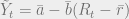
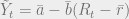
The IS Curve describes how output, , changes in response to a change in the real interest rate, . It is given by: . Here, is a demand shock, is the marginal product of capital (you can think of this as the return that a businesses in the economy will receive if they buy one more machine). A good way to think about the real interest rate, , is the return that businesses would receive if they put their money in a savings account. Therefore if the real interest rate increases, then businesses will be more likely to put their money in a savings account rather buying a new machine, and investment will decline.

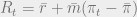
The second equation is the monetary policy (MP) curve, which describes how the central bank changes the real interest rate in response to changing inflation: . Here, is the actual inflation rate this year, and is the central bank’s inflation target. This rule says that as inflation increases, the central bank will raise interest rates (with the intention of decreasing investment, and therefore cooling the economy off).

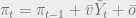
The third equation is the aggregate supply (AS) curve. This equation describes how firms change prices, and therefore it describes how inflation changes over time. It is given by: . Here, is an inflation shock, and is the inflation rate last year. This equation says that if short-run output, , increases, then businesses are faced with a lot of extra demand, so they will raise prices. The story that we tell is that if businesses have a lot of demand, then they can raise prices by more than usual without fear of losing customers. If businesses are raising prices, then there is more inflation.

Taken together, we have:
IS: 
MP:
AS: 

We can combine the IS & MP curves to get the aggregate demand curve. Now we have our two equations:
AD: 
AS: 

Aggregate demand (AD) combines two relationships. First, if inflation rises, the central bank will increase interest rates. Second, if interest rates rise, investment will fall, leading to a decrease in output. Therefore, as we can see in the AD curve, if inflation increases, output will fall. Note that this is not just a law of nature – the reason that output falls when inflation rises is due to the policy of the central bank. This will be very important in future posts.

Graphically:

This summarizes the model as presented in Jones (2014). However, this analysis completely neglects the zero-lower bound, i.e. the fact that nominal interest rates on savings accounts can’t go below zero (if interest rates were negative, then people would just keep their money at home rather than put it in the bank). Therefore, if the MP curve calls for the central bank to set a very negative real interest rate, the central bank will not be able to do it – this problem is called a liquidity trap, and it’s where policymakers around the world have found themselves stuck ever since 2009.

Because the model, as currently derived, does not take this possibility into account, it features a misspecified monetary policy curve (and therefore a misspecified AD curve, since MP is used to derive AD). How to fix the MP curve to allow for the fact that nominal interest rates can’t go negative is the subject of my next post.